Diogo Almeida, Nate Sauder, Sasha Targ, Vrushank Vora
Table of Contents
About This Post
The following blog post was the collaborative output of the our Deep Learning (DL) reading group. We seek to be thoughtful about every aspect of our reading group and iteratively discover/measure/optimize the parameters of its success. More is written here about what we have learnt. Please email info@topos.house if you are interested in optimizating both deep learning models and collaborative learning simulatenously. (:
Summary
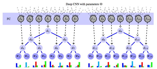
Paper: Deep Neural Decision Forests (dNDFs), Peter Kontschieder, Madalina Fiterau, Antonio Criminisi, Samuel Rota Bulò, ICCV 2015
The function spaces of neural networks and decision trees are quite different: the former is piece-wise linear while the latter learns sequences of hierarchical conditional rules. Accordingly, it feels intuitively appealing to combine those function spaces to leverage the strengths of both.
-
Each activation of the final layer of the neural network corresponds to the routing probability of going left or right in the decision tree
-

-
Each leaf is associated with a probability vector over the classes, e.g. {cat : 0.84, dog : 0.06, bird : 0.10}

-
The probability of a leaf node is the product of the (routing) probabilities of taking each left/right choice
-
The output of a deep NDF is the weighted sum of each probability vector with its routing probability
As such, the network output is a form of soft attention1 over a constant (but optimized) set of probability vectors where that attention happens to be computed with a tree. The are trained using regular gradient descent while the optimal probability vectors can be solved using convex optimization before each epoch.
Top Thoughts
- The most notable thing about this paper is the results. While beating the standard GoogLeNet’s 6.67% top-5 error on ImageNet is impressive with dNDF.NET’s 6.38%, the accuracy with a single model was also significantly better (7.84% vs 10.07%). Perhaps most interestingly, even the shallowest dNDF (a 12 layer deep model) of the model had better accuracy than GoogLeNet (a 22 layer deep model). It would be very interesting to see if the 12 layer model could beat GoogLeNet if trained without the extra layers, or if having extra layers on top somehow regularizes the model to generalize better.
- Because of the extremely different output layer, we should expect qualitatively very different embeddings from this model, possibly ones that represent the hierarchical nature of the decision forest. It would be interesting to explore the kinds of properties that these embeddings exhibit and to think about what kind of downstream tasks could benefit from these embeddings.
- We can visualize the kinds of splits at each node of the tree by identifying top images for each sigmoid neuron. Thereby, we might be able to explore the hierarchical nature of the dataset which is particularly useful when the domain is foreign to the DL practitioner.
MNIST Experiments
The results in this paper were very promising; however, many factors were changed at the same time. So, we constructed and ran experiments to isolate where the benefits came from.
tn.HyperparameterNode(
    "model",
    tn.SequentialNode(
        "seq",
        [tn.InputNode("x", shape=(None, 28 * 28)),
         tn.DenseNode("fc1"),
         tn.DropoutNode("do1"),
         tn.ReLUNode("relu1"),
         tn.DenseNode("fc2"),
         tn.DropoutNode("do2"),
         tn.ReLUNode("relu2"),
         tn.DenseNode("fc3", num_units=10),
         tn.SoftmaxNode("pred")]),
    num_units=512,
    dropout_probability=0.5,
    inits=[treeano.inits.XavierNormalInit()])
The baseline network for MNIST. 2
I. Softmax Attention on Weight Matrix
The first thing we tried was soft attention over a weight matrix. That averaged result was then converted into a probability vector via another softmax. It was easily implemented using the built-in components of most neural network libraries. It performed much worse than a baseline network.
tn.HyperparameterNode(
    "model",
    tn.SequentialNode(
        "seq",
        [tn.InputNode("x", shape=(None, 28 * 28)),
         tn.DenseNode("fc1"),
         tn.ReLUNode("relu1"),
         tn.DropoutNode("do1"),
         tn.DenseNode("fc2"),
         tn.ReLUNode("relu2"),
         tn.DropoutNode("do2"),
         # ONLY DIFFERENCE: replace ReLU with softmax
         tn.SoftmaxNode("soft_attention"),
         tn.DenseNode("fc3", num_units=10),
         tn.SoftmaxNode("pred")]),
    num_units=512,
    dropout_probability=0.5,
inits=[treeano.inits.XavierNormalInit()])II. 2-Step Optimization
The next thing we tried was optimizing the final layer independently of the rest of the network, as in the paper.
We implemented the convex optimization of the final layer using SGD (the Adam learning rule, specifically, just as the rest of the MLP was optimized with) and going through 10 epochs optimizing the final layer for every epoch of the rest of the network.
On the baseline network, there was not a large difference in accuracy. However, it took a lot longer to optimize due to the extra steps in the optimization.
The 2-step optimization in combination with the network from section I. improved its performance up to baseline levels. Thus, it seems like the double softmax negatively affected the optimization of the previous network which the 2-step optimization helped undo.
III. Softmax Attention on Probability Matrix
Realizing that soft attention over a weight matrix and converting to a probability afterwards is very different from soft attention over a probability matrix, we implemented the latter next.
This was done by creating a weight matrix, taking a softmax across each row, then taking the dot product of the soft attention probabilities with this probability matrix (source).
Performed as well as the baseline but converged significantly slower. Combining this with the 2-step optimization had similar results, in both accuracy and convergence rate.
IV. Tree Attention on Probability Matrix
We then implemented a differentiable decision tree module that inputs probabilities for splitting at each node and outputs a probability of landing at each leaf.
We implemented it once in Theano (source), which was very easy but not very efficient and took very long to compile for large trees and once as a custom Op in numpy (source).
# iterate over all splits in the tree, pre-calculated
# by left and right boundaries, and  multiply left subtree
# nodes by probability of going left (and likewise for right)
for idx, (l, m, r) in enumerate(tree):
  res[:, l:m] *= probabilities[:, idx, np.newaxis]
res[:, m:r] *= (1 - probabilities)[:, idx, np.newaxis]We had some issues getting this model to train effectively. Some things we found were that:
-
The model was more sensitive to learning rate, which needed to be increased from Adam’s default
-
Batch Normalization before the sigmoids for the leaf probabilities helped
-
Dropout before the tree seemed harmful
The model successfully trained with this combination of tricks. However, neither standard SGD or the 2-step optimization improved upon the baseline.
V. In-network Ensembling
The final trick mentioned in the paper that we hadn’t yet implemented (at least approximately) was multiple trees and randomly sampling which tree to optimize. We used 10 output layers for this part and applied it to both the softmax and the tree models.
We implemented this by making the softmax and decision tree modules polymorphic to higher dimensional tensors, adding an additional dimension in the network representing which output layer is being used, and then either sampling one of the output layers to optimize at train time or taking the average of the predictions at test time.
# create activations for 10 trees
# each with 63 split nodes (thus 64 leaves)
tn.DenseNode("fc2", num_units=63 * 10),
# convert activation into split probability
tn.SigmoidNode("sigmoid"),
# reshape to rank 3 tensor
tn.ReshapeNode("reshape", shape=(500, 63, 10)),
# convert split probability to leaf probability along axis 1
dNDF.SplitProbabilitiesToLeafProbabilitiesNode("tree"),
# swap axes so that ensemble axis is axis 1
tn.SwapAxesNode("sa", axes=(1, 2)),
# apply soft attention over probability vectors
dNDF.ProbabilityLinearCombinationNode("to_probs", num_units=10),
# at train time, select a single tree
dNDF.SelectOneAlongAxisNode("s1", axis=1),For both softmax attention and tree attention with 2-step optimization, this similarly did as good as the baseline model. Without 2-step optimization though, this caused significantly worse performance, possibly because the output layers are optimized 1/10th as much.
VI. Conclusions
MNIST is a toy dataset and insights are especially questionable with a relatively shallow MLP on it, so it is difficult to make conclusions on how good these techniques would work on a more complex dataset. We used this more as a test bed to make sure everything works and to get a rough feel for how robust these tricks are to different hyperparameters and network topologies. Since both softmax attention and tree attention performed similarly to baseline models, this seemed promising enough to try on (slightly) larger datasets.
Based on these experiments alone though, none of these tricks (without any tuning) seemed to result in significant benefits. There was no clear advantage of tree attention over softmax attention.
CIFAR Experiments
We next decided to test both softmax and tree attention on CIFAR-10 and CIFAR-100.
We found that with the deeper network (8-layers)3 used, both types of attention led the network not to train. Using Batch Normalization throughout the network and increasing the learning rate solved that issue.
On CIFAR-10, both types of attention performed worse than a baseline network with Batch Normalization:
| Model | Accuracy (%) |
|---|---|
| Baseline | 90.38 |
| Softmax Attention | 89.91 |
| Tree Attention | 89.84 |
One hypothesis for why the tree was so effective on the ImageNet dataset is that the highly hierarchical label space lends itself well to trees, which doesn’t seem important for 10-class classification problems such as MNIST and CIFAR-10. We thus tried running some models on CIFAR-100, though this led to similarly unpromising results:
| Model | Accuracy (%) |
|---|---|
| Baseline (embedding size=192) | 62.50 |
| Softmax Attention (embedding size=192) | 26.21 |
| Softmax Attention (embedding size=2047) | 55.02 |
| Tree Attention (embedding size=127) | 47.68 |
| Tree Attention (embedding size=2047) | 52.84 |
Tree attention seemed initially promising compared to using a softmax for smaller embedding sizes4, but for a larger embedding size, that benefit was no longer observed, and performance did not reach that of the baseline.
And More
Since this was generated collaboratively, we also have a document outlining questions, answers, explanations, references, thoughts, and more here. Feel free to comment on it.
-
Soft attention can be seen as either an intelligent weighted average, or treating the decision trees stochastically and taking the expected vector. See Neural Machine Translation by Jointly Learning to Align and Translate for more. ↩
-
The architecture was based on the one from Scalable Bayesian Optimization Using Deep Neural Networks. ↩
-
Note that the size of the tree embeddings had to be a power of 2 minus 1, because the binary tree is balanced. ↩